Background
Constructing an isosurface of a scalar field essentially constitutes finding those set of point on the grid that share an isovalue and connecting those points. Many explanations have been written on the topic and I warmly invite the reader to study the excellent work of Paul Bourke on this topic.
Algorithm
PyTessel uses the marching cubes algorithm. In this algorithm, the scalar field is represented as a set of point on a (typically regular) grid. Each octet of grid points thus represents a cube. For each of the 8 vertices in each cell, it is determined whether the value of the function is larger or smaller than the isovalue. If for one vertex the value is larger than the isovalue and for another vertex the value smaller than the isovalue, then the isosurface has to cut the edge that is shared by the two vertices.
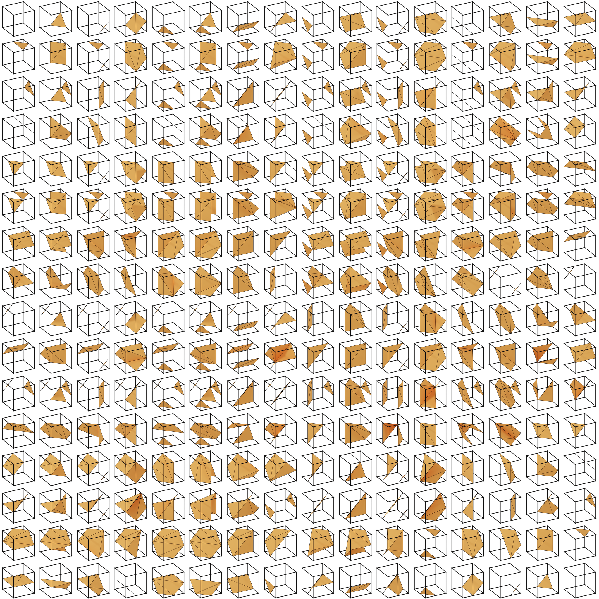
Given eight vertices per cube, there are only \(2^{8}=256\) possibilities of how a scalar field can interact with each cube. An overview of all these possibilities is provided in the image below. Note that within this set of 256 possibilities, there are only 15 unique results as the majority of the results are linked by a symmetry operation such as a rotation. All these 256 different ways by which the scalar field can interact with each cell are stored in a pre-calculated table by which the resulting list of edge intersections and the polygons that originate from these intersections can be readily found. The exact position where the isosurface intersects each edge is determined using trilinear interpolation.
The algorithm essentially proceeds as follows:
The space wherein the function is evaluated is discretized into small cubes.
For each vertex on these cubes the function is evaluated and it is determined whether the value for the function at each of the vertices is larger or smaller than the isovalue. This leads to a number of edge intersections for each cube from which the polygons (triangles) for each cube can be established.
All polygons are gathered to form the threedimensional isosurface.
It should be noted that this algorithm can be executed in a highly efficient fashion using trivial parallellization as the result for each cube is completely independent from all the other cubes. It turns out that the generation of the scalar field, which by itself is also a highly parallellizable step, is typically the most time-consuming.